解几何题调研
Diagram Understanding in Geometry Questions
- AAAI 2014 论文地址
- 本文提出了一个叫做 G-ALIGNER 的 Image Parse 的工具,并证明了它使用的估价函数是次模函数。
- 估价函数介绍
- 设 表示题目文本中提到的元素集合, 是图片中初步提取后的所有 primitives 集合。本论文默认 已经得到,现在要找一个最优的子集 以准确地表达图片信息。
- 引入一个 表示该图上的 primitive 是否与指定文本元素对应。 ,可以将求一个最优子集 转化为求一个最优的矩阵 。
- 对于一个可能的集合 ,估价函数 设计成三个部分:
- 所选 primitives 与实际的图像之间的重合程度
- 所选 primitives 能构成更高相关性 visual element 的程度
- 所选 primitives 与文本的对应关系 ,其中 表示冗余成分。
- 可以证明, 是次模函数。
- 求解步骤
- 用 Hough transform 提取 primitives,用 Harris Corner detectors 检测 Corners。
- 优化时采用很暴力的方式:初始时设 ,.每次枚举 ,把 的 加入 ,直到增量 为止。
Solving Geometry Problems: Combining Text and Diagram Interpretation
- EMNLP 2015 论文地址
- 提出了一个 GEOS 系统,把文本和图片变成 形式语言(logical expression)再推理。
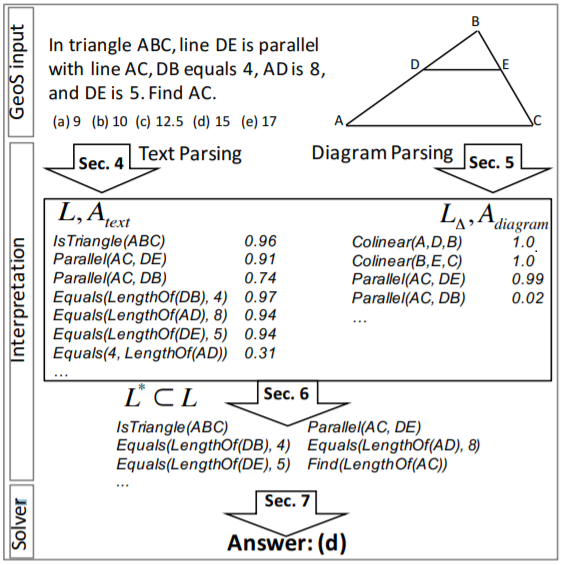
- logical expression 的定义
- 它是一阶逻辑语言(first-order logic),包含以下四种内容:
- constants :已知的量或实体。例如
5。 - variables:未知的量或实体。例如
x,CE。 - predicates:几何或算术的关系。例如
Equals,IsDiameter,IsTangent。 - functions:几何物体的性质或者算术运算。例如
LengthOf,SumOf。
- constants :已知的量或实体。例如
- 定义 Literal 是 predicates 的应用实例,如
isTriangle(ABC) - 定义 Logical formulas 是以上内容和 existential quantifiers,conjunctions 的组合,如:
1
∃x, IsTriangle(x)∧IsIsosceles(x)
- 它是一阶逻辑语言(first-order logic),包含以下四种内容:
Transformers as Soft Reasoners over Language
- 论文地址
- 挖坑
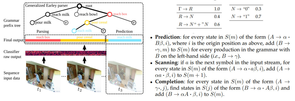
A Generalized Earley Parser for Human Activity Parsing and Prediction
-
This paper is an extension of previous ICCV and ICML papers. 1TPAMI 2020 Address
-
Earley Parser is a classical method to parse CFG, while it can not tackle the non-Markovian and compositional properties of high-level semantics. This paper generalize the Earley parser to solve sequence data by only given an arbitrary probabilistic classifier.
-
This Generalized Earley Parser combined detection, parsing and future predictions together, which is really generic and applicable. It finds the optimal (maximizing the joint probability) segmentation and label sentence according to both a symbolic grammar and a classifier output of probabilities of labels for each frame.
-
Brief introduction for EARLEY PARSER
- Early parser takes a sentence with length as input, and find out this CFG.
- It is similar with LR parser. There are three main process:
- Prediction: For each , add if exists.
- Scanning: If and the next character is , add .
- Completion: If appears, change to .
- l=k1k2 k3
- An sample
-
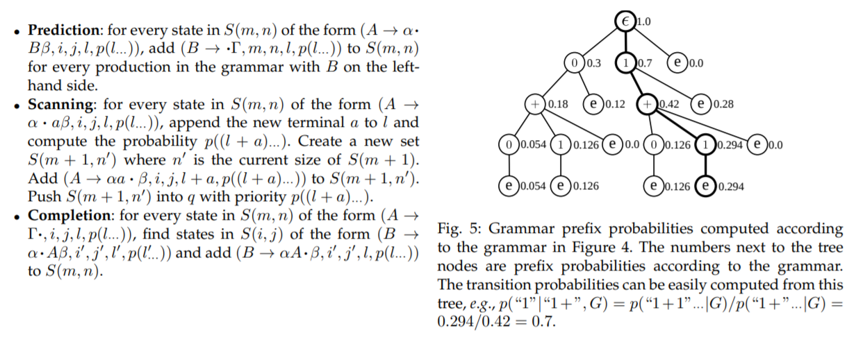
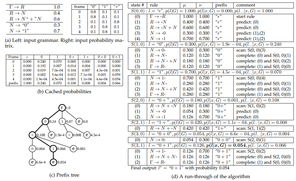
GENERALIZED EARLEY PARSER
- Consider a sequence with length , Generalized Early parser takes an probability matrix as input, and output sentence of labels that best explains the data according to a grammar G, where each label corresponds to a segment of sequence.
- Parsing Probability
- The parsing probability is computed in a dynamic programming fashion.
- Consider whether this frame is a new frame with label . The previous frames can be labeled as either or :
- x [0:t] = xxxxxxxx…
- l = k1k2k3…
- l=1+…
- l=1+ 1
- l=1+1… / l=1+…
- Prefix Probability
- Then we compute the prefix probability . Once the label is observed (the transition happens), l becomes the prefix and the rest frames can be labeled arbitrarily.
- In practice, the probability decreases exponentially as increases and will soon lead to numeric underflow. So we should solve it with .
- Posterior Probability
- Transition probability can be calculated by: $$p\left(k | l^{-}, G\right)=\frac{p(l \ldots | G)}{p\left(l^{-}, | G\right)}$$.
- So we can modify the posterior of Parsing Probability by:
- And the posterior of Prefix Probability is:
- An sample
-
Generalized_Earley_Parser_Sample
Closed Loop Neural-Symbolic Learning via Integrating Neural Perception, Grammar Parsing, and Symbolic Reasoning
- ICML2020. Propose a Neural-Grammar-Symbolic Model (NGS).
- Learning neural-symbolic models with RL approach usually converges slowly with sparse rewards. The author proposes a novel top-down back-search, which can also serve as Metropolis-Hastings sampler (a sampling method in MCMC).
- Model Inference
- Let be the input (e.g.an image or question), be the hidden symbolic representation, and be the desired output inferred by .
- Neural Perception: Map to a normalized probability distribution of the hidden symbolic representation :
- Grammar Parsing: Find the most probable that can be accepted by the grammar: . We use Generalized Early Parser doing the grammar parsing.
- Symbolic Reasoning: Given the parsed symbolic representation , performs deterministic inference with and the domain-specific knowledge to predict :
- Learning Details
-
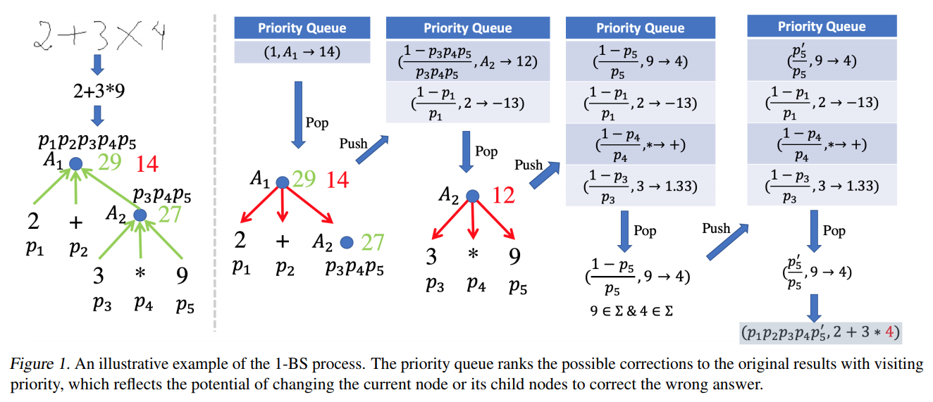
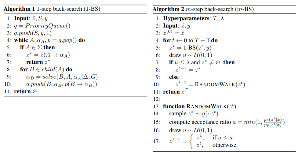
1-STEP BACK-SEARCH
- Previous methods using policy gradient to learn the model discard all the samples with zero reward, but 1-STEP BACK-SEARCH can correct wrong samples and use the corrections as pseudo labels for training.
- In the 1-BS, assume that only one symbol can be replaced at a time. Given , the 1-BS gradually searches down the reasoning tree starting from the root node to the leaf nodes and wants to find the most probable correction at one-step distance.
- During this process, maintain a priority queue storing 3-tuple : current node, current expected value (If the value of changes to , will execute to the ground-truth answer ) and the visiting priority (probability).
- When transformation, enumerate each child of and calculate expected value such that . New tuple: .
- p\left(A \rightarrow \alpha_{A}\right)=\left\{\begin{array}{ll} \frac{1-p(A)}{p(A)}, & \text { if } A \notin \Sigma \\ \frac{p\left(\alpha_{A}\right)}{p(A)}, & \text { if } A \in \Sigma \and \alpha_{A} \in \Sigma \end{array}\right.
-
MAXIMUM LIKELIHOOD ESTIMATION
- For a pair of , we know
- The learning goal is to maximize . By taking derivative:
- Computing the posterior distribution is not efficient.
- We only need to consider , which is usually a small part.
- So we want to sample from efficiently using Markov chain Monte Carlo.
-
m-BS AS METROPOLIS-HASTINGS SAMPLER
- Use Metropolis–Hastings algorithm to sampe from the probability distribution.
- Detailed balance is a sufficient condition to get a stationary distribution. To contruct a valid , we use acceptance-rejection model and the ratio is so that .
-
- Assume that the transition probability during Random Walk is Poisson distribution. , where is usually set to .
- So we know
-
Algorithm for 1-BS and m-BS
-
COMPARISON WITH POLICY GRADIENT
-
Treat as the policy function and the reward given can be written as
-
Similarly,
-
-
Among the whole space of , only a very small portion can generate the desired , which implies that the REINFORCE will get zero gradients from most of the samples.
-
-
 wechat
 alipay