《混合现实》知识整理

During $2019.9 \sim 2020.1$ ，I was involved in the Mix-Reality class guided by Hujun Bao.

The topic in this class is similar with computer vision. I’m really regretful because I didn’t listen to Mr. Bao’s class carefully, even though he explained the knowledge points carefully.

Mr. Bao sent me a book written by himself. I must read it when I’m free.

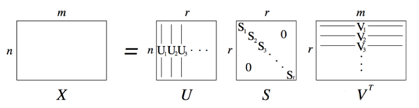
Singular Value decomposition(SVD)

a factorization of a normal matrix, extended from eigendecomposition.
$A_{n \times m} = U_{n \times n}\Sigma_{n \times m}V^T_{m \times m}$ $A_{n \times m} = U_{n \times n} Σ_{n \times m} V_{m \times m}^{T}$
- $(A^TA)v_i = \lambda_iv_i$
- singular values: $\sigma_i = \sqrt{\lambda_i}$
- $u_i=\frac{1}{\sigma_i}Av_i$
One can easily verify that the square matrix also satisfies this definition(the same as eigendecomposition).
$U,V$ are orthogonal matrices
Usually we set $r \in (0,rk(A)]$ to approximate SVD.

Transfomation in 2D

Name	Function	Preserve	DOF
Isometries	rotation, translation	distance	$3$
Similarities	[above], scale	ratio of lengths, angles	$4$
Affinities		parallel lines, ratio of areas and lengths	$6$
Projective		cross ratio of 4 collinear points, collinearity	$8$

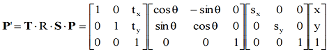
Rotation+Scaling+Translation
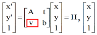
Affinities
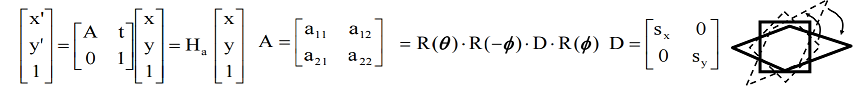
Projective
- find $H$ $H$
  - Due to projective transformation, they are in 3D Homogeneous Coordinates and $x' \times Hx = 0$ .
  - Rewrite $9$ parameters from $H$ in a column vector $h$ . For one pair of points, it can be derived that $A_{3\times9}h_{9 \times 1}=0$ . Note that although there are $3$ equations, only $2$ of them are independent. So finally we can acquire that $A_{2N\times9}\cdot h=0$
  - Use SVD to solve this equation: $A=U_{2N\times9}\Sigma_{9\times9}V^T_{9\times9}$ . $h$ is is the last column of $V^T$ .
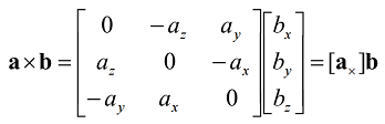
Cross in Matrix

Camera Model

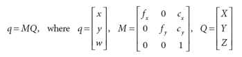
Pinhole camera
- Because the point is not exactly at the center, we should add shift parameters $c_x$ and $c_y$ . So that $x'=f_xx+c_x, y'=f_yy+c_y$ .
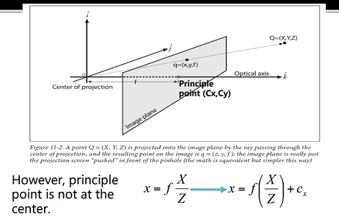
- Why the aperture cannot be too small?
  - Less light passes through
  - Diffraction effect
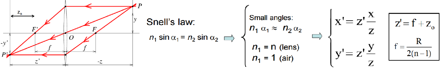
Lenses
- For thin lense:

Camera Calibration

intrinsic parameters
- From Pinhole Camera Model, totally $4$ parameters. Use the trick of Homogeneous Coordinates, finally:
extrinsic parameters
- rotation and translation
- $6$ parameters: $(\theta, \phi, \psi, c_x, c_y, c_z)$
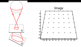
distortion parameters

Radial distortion
```
  ![](Mix-Reality/camera5.png)
```
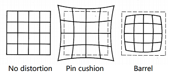
Tangential distortion
```
  ![](Mix-Reality/camera7.png)
```
- $5$ parameters: $(k1,k2,k3,p1,p2)$

Camera Calibration
- Without distortion, the transform matrices are as follows ( $s$ is the Skew parameter):
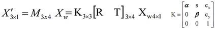
- parameters number: $5+3+3=11$ . Need $6$ correspondences.
Homogeneous $M \times N$ Linear Systems
- $Ax=0$ , $A_{M \times N}, M > N$
- To find non-zero solution, Minimize $|Ax|^2$ under the constraint $|x|^2=1$ .
- A possible method: Direct Linear Transformation
- General method for Calibration Problem: Compute SVD decomposition of $A$ , the last column of V gives $x$ .
- Degenerate cases
  - Points cannot lie on the same plane.
  - Points cannot lie on the intersection curve of two quadric surfaces.
Taking Radial Distortion into Account
- nonlinear
- Methods
  - Newton Method
  - Levenberg-Marquardt Algorithm
- The latter doesn’t require the computation of $H$ .

Stereo-view Geometry

Sets of parallel lines on the same plane lead to collinear vanishing points.
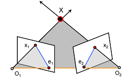
Epipolar Geometry 对极几何
Epipolar Constraint
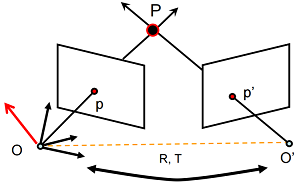
- Denote $p=K[I,0]P$ and $p'=K[R,T]P$ .
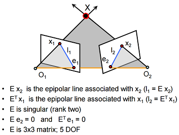
- Let $x=K^{-1}p$ , finally we get that $x^T \cdot [T \times (Rx')] = 0$ , which is called Epipolar Constraint. It means that vector $x^T$ , $T$ and $Rx'$ are coplanar.
- Denote $E=T \times R$ , then $x^TEx'=0$ , $E$ is called Essential Matrix.
- Properties about Essential Matrix
- Write back $K$ (may different between cameras), $F$ is called Fundamental Matrix.
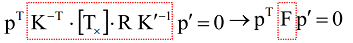
  - Properties about Fundamental Matrix is similar to essential matrix. $7$ DOF.
Solve for Fundamental Matrix
- $Wf = 0$ $W f = 0$ ( $f_{9 \times 1}$ $f_{9 \times 1}$ collects the parameters in $F$ $F$ ).
  - If $rk(W)=8$ : exists unqiue $f$ .
  - If $rk(W)>8$ : find $\hat F$ calculated by SVD.
- Note that $F$ ’s rank is $2$ but $\hat F$ may not. Second equation: $||F-\hat F|| =0$ and $det(F)=0$
- Normalization
  - Transform one image first before calculating $F$ .
  - Find a transform that: Origin (1) centroid of image points. (2) Mean square distance of the data points from origin is $2$ pixels.

Stereo systems

Some applications
- Stereo vision: Estimate the position of $P$ given the observation of $P$ from two view points.
- Triangulation: Intersecting the two lines of sight gives rise to $P$
Making image planes parallel
- Goal: Estimate the perspective transformation $H$ that makes the images parallel.
- To be continued…
Correspondence problem
- Correlation Methods
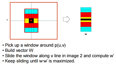
- Smaller window
  - More detail
  - More noise
- Larger window
  - Smoother disparity maps
  - Less prone to noise
- To be continued…

Image Processing

Filters
- goals
  - Extract useful information from the images
  - Modify or enhance image properties
- Gaussian Filters
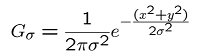
  - Rule of thumb: set filter half-width to about $3\sigma$
  - Separable kernel; Convolution with self is another Gaussian
- Median and Mean filter
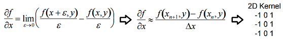
Differentiation
Sub-sampling
- Problem: Aliasing
- Sampling Theorem (Nyquist)： When sampling a signal at discrete intervals, the sampling frequency must be $2f_{max}$ ( $f$ is frequency).
Edge Detection
- Edge: a location with high gradient
- Most widely used method: Canny Edge Detection
  1. Gaussian smoothing
  2. Derivative of Gaussian
  3. Find magnitude and orientation of gradient
  4. Extract edge points: “Non-maximum suppression”
  5. Linking and thresholding “Hysteresis”
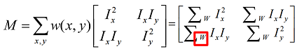
Harris Corner Detector
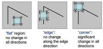
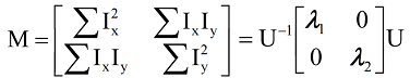
- Denote $E(u,v)=\sum \limits_{x,y} w(x,y)[I(x+u,y+u)-I(x,y)]^2$ . The corner has bigger $E(u,v)$ .
- Using bilinear approximation, we can derive that:
  - $\lambda1 \sim \lambda2$ : Corner
  - $\lambda1 \gg \lambda2$ : Edge
- Set $\rm R=det(M)-k \cdot Trace(M)$ , use $R$ to judge corners ( $k \in [0.04,0.06]$ ).
- Property: Rotation invariance