《计算机视觉》知识整理
计算机视觉》考前知识点整理。参考:这个网站。
引言
- Gestalt Laws(格式塔法则):出发点是形。
- Law of Proximity: 接近的物体容易被感知成同一组。
- Law of Similarity: 将相似的物体感知成同一组的部分。
- Law of Good Continuation: 沿着元素暗示的弧方向走。
- Law of Closure: 人们会把不完整的个体看成是一个整体的形状。
- Law of goodform : 希望图片由几个规则图形组成。
- Law of Figure/Ground: 区别前景和背景。
- 什么是计算机视觉?
- 根据场景的图像实现场景中对象信息的恢复和利用。
- 五大研究内容
- 输入设备
- 底层视觉(图像处理)
- 中层视觉(恢复场景,2.5 维)
- 高层视觉(三维重建)
- 体系结构
- Marr 视觉表示框架
- 信息处理分析的三个层次
- 计算层:目的,策略。
- 表示和算法层:实现这个计算。
- 实现层:物理上实现。
- 视觉表示框架:
- 第一阶段 (Primal Sketch):将输入的原始图像进行处理,抽取图像中诸如角点、边缘、纹理、线条、边界等基本特征, 这些特征的集合称为基元图;
- 第二阶段 (2.5D Sketch):指在以观测者为中心的坐标系中, 由输入图像和基元图恢复场景可见部分的深度、法线方向、 轮廓等,这些信息包含了深度信息,但不是真正的物体三维表示,因此被称为二维半图;
- 第三阶段 (3D Model):在以物体为中心的坐标系中,由输入图像、基元图、二维半图来恢复、表示和识别三维物体。
- 信息处理分析的三个层次
二值图像
- 几何特性
- 面积(零阶矩),区域中心(一阶矩)。
- 方向(求方向用最小二乘法),伸长率 ,密集度
- 欧拉数 (亏格数, genus) = 连通分量数减去洞数
- 常用距离:欧几里德距离 (Euclidean) ,街区距离(block) ,棋盘距离,Minkowski 距离(p-norm distance)。
- 投影计算
- 定义:给定一条直线,用垂直该直线的一簇等间距直线将一幅二值图像分割成若干条,每一条内像素值为1的像素的数量。
- 水平投影,垂直投影。
- 对角线投影:对角线标号
- 连通区域
- 连通分量标记的序贯算法(二重循环+并查集)
- 区域边界跟踪算法
- 从左到右、从上到下找到左上角的起点 ,初始化 是它左侧的点。
- 从 开始围绕 逆时针旋转,设找过的点编号为 。
- 当的值是 时停止,设 ,重复操作 直到结束。
边缘和边缘检测
- 模板卷积
- 四种最主要的不连续:
- 表面法向量的不连续
- 深度的不连续
- 表面颜色的不连续
- 光照的不连续
- 边缘检测基本思想:函数导数反映图像灰度变化的显著程度。一阶导数的局部极大值,或二阶导数的过零点。
- 基于一阶导数的边缘检测
- 幅值
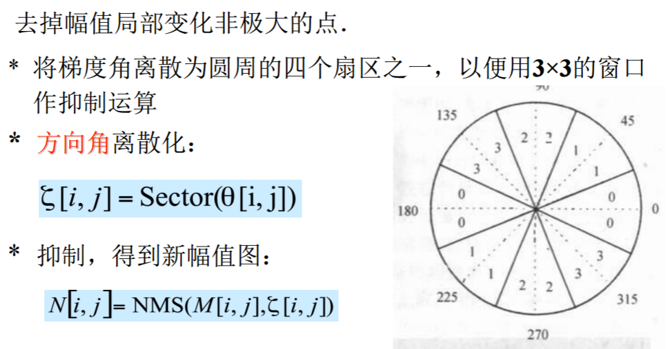
- 梯度方向:
- 用差分近似偏导数:Roberts交叉算子,Sobel算子(左边 中间全 ),Prewitt算子(左边 ,中间全 )
- 基于二阶导数的边缘检测
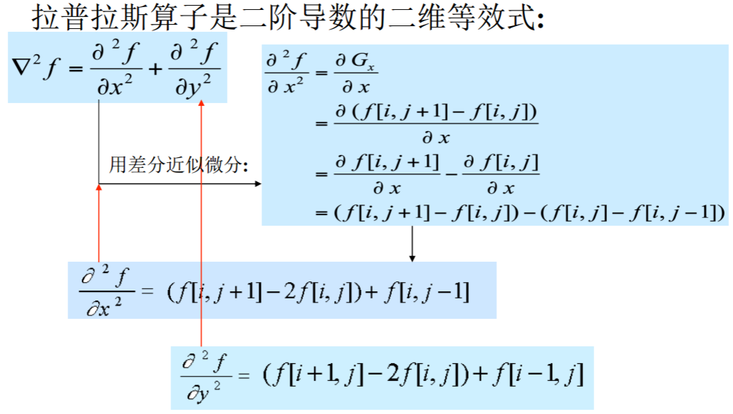
- 拉普拉斯(Laplacian)算子
- LoG(Laplacian of Gaussian)边缘检测算法
- 平滑滤波器是高斯滤波器。
- 采用拉普拉斯算子计算二阶导数。
- 边缘检测判据是二阶导数零交叉点并对应一阶导数的较大峰值。
- 使用线性内插方法在子像素分辨率水平上估计边缘的位置。
- 先做卷积再求二阶导 和 先对高斯滤波求二阶导再卷积 等价。
- 拉普拉斯(Laplacian)算子
- 基于一阶导数的边缘检测
- Canny 边缘检测器
- 用高斯滤波器平滑图像
- 用一阶偏导有限差分计算梯度幅值和方向
- 对梯度幅值进行非极大值抑制(NMS)
- 用双阈值算法检测和连接边缘
- 高阈值:必然是边缘
- 低阈值:必须和高阈值连通才算边缘
局部特征 Local Feature
-
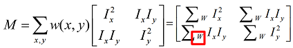
Harris 角点检测
- Denote . The corner has bigger .
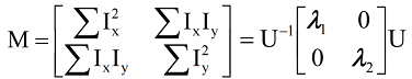
- Using bilinear approximation, we can derive that:
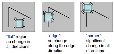
- : Corner
- : Edge
- Corner Response , use to judge corners ().
- Algorithm
- Find points with large corner response function R (R > threshold) .
- Take the points of local maxima of R
- Property
- Rotation invariance 旋转不变性
- Partial invariance to affine intensity change 灰度仿射不变性
- But: non-invariant to image scale!
-
Scale Invariant Detections
- Given: two images of the same scene with a large scale difference between them.
- Goal: find the same interest points independently in each image.
- Solution: search for maxima of suitable functions in scale and in space (over the image).
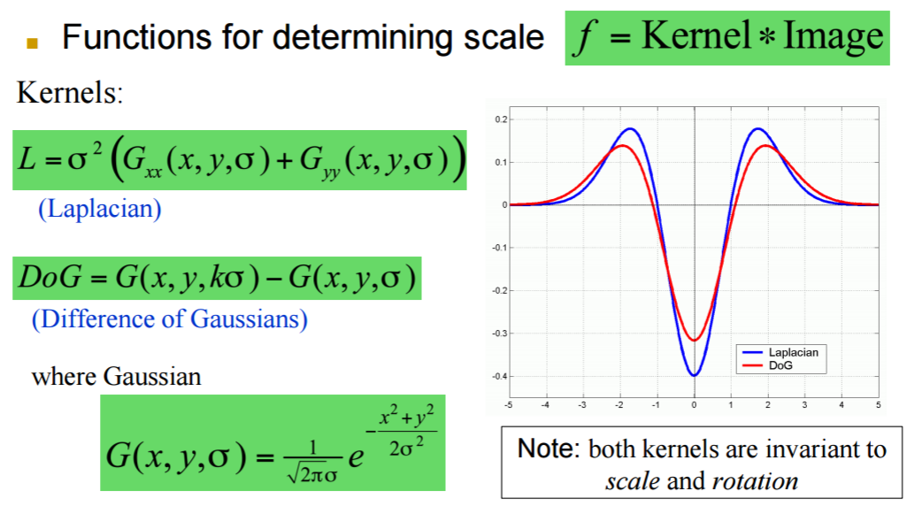
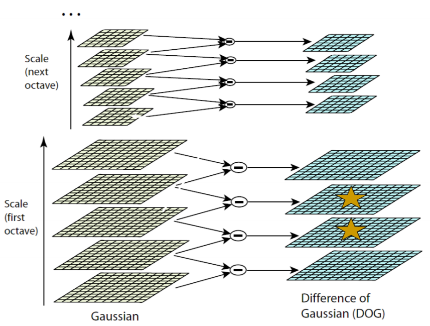
-
Harris-Laplace: DoG:
-
SIFT描述子的计算
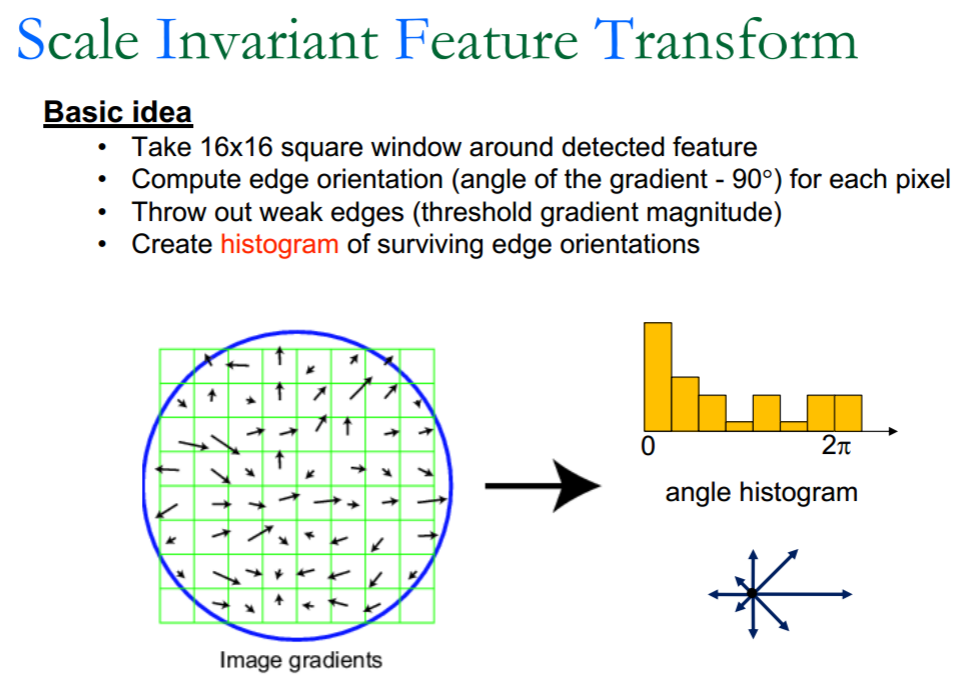
- Full Version
- Divide the 16x16 window into a 4x4 grid of cells.
- Compute an orientation histogram for each cell
- 16 cells * 8 orientations = 128 dimensional descriptor
- SIFT Feature
- Descriptor: 128-D: Normalized to reduce the effects of illumination change.
- Position: (x, y)
- Scale: Control the region size for descriptor extraction.
- Orientation: To achieve rotation-invariant descriptor.
- Merit
- Desired property in invariance in changes of scale, rotation, illumination, etc.
- Highly distinctive and descriptive in local patch. Especially effective in rigid object representation.
- Drawback
- Time consuming for extraction
- Poor performance for un-rigid object. Such as human face, animal, etc.
- May fail to work in severe affine distortion.
- Full Version
曲线
-
和边缘检测的关系:将边缘连接起来就可以知道一个物体在二维平面上的投影边界,称这一边界为轮廓。
-
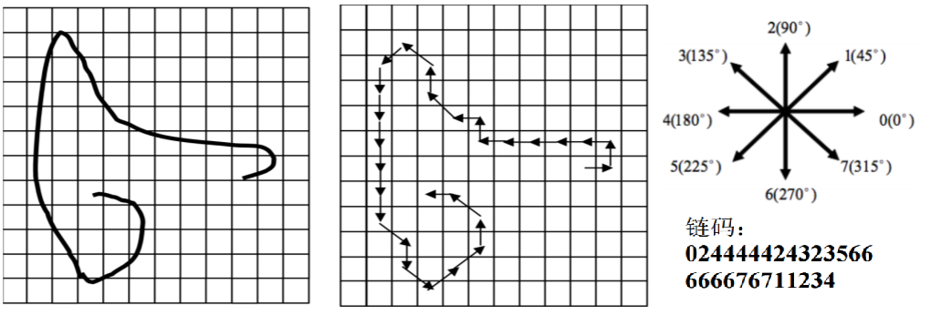
链码用相邻边缘点组成的方向序列来表示边缘
- 4-连通对应四方向链码
- 8-连通对应八方向链码
-
分线段 (多边形) 拟合:Douglas-Peucker算法 [Douglas73]
- 对每一条离散曲线的首末点虚连一条直线,求所有点与直线的距离,并找出最大距离值 ,用 与阈值 相比:
- 若 ,这条曲线上中间点全部舍去;
- 若 ,保留dmax对应的点,并以该点为界,把
曲线分为两部分,对这两部分重复使用该方法。
-
Hough变换
- Hough变换是一种特征提取技术,基于投票 (Voting) 原理的参数估计方法,用来检测直线、圆等形状。
- 基本想法:图像中每一点对参数组合进行表决,赢得多数票的参数组合为胜者。
- 检测直线
- 原图的一个点 上会经过很多 的直线。我们写成 的形式,做 的映射。
- 这样,原图的每一个点就转换成了参数空间中的直线。
- 避免垂直直线所带来的问题,通常采用极坐标表示: 空间到 空间的变换。
- 在参数空间开一个累加器。对于原图的每个点,把参数空间对应直线经过的点累加器都加一。最终我们再把参数空间里值最大的累加器点变换回原图,就可以表征原图最有可能的直线了。
- 检测圆弧
- 一个圆弧有 三个参数。
- 由 得变换规则 :(参数空间是 )
- 对于原图的每个点计算梯度角 ,并在对应参数空间维护累加器。做完后我们就得到了最有可能的圆心坐标。很容易反求出 。
人脸识别
- Principal component analysis
- It is a linear transformation that chooses a new coordinate system for the data.
- PCA 定义
- 数据在 维空间
- 我们想要找一些投影方向 ,使得 且投影值 的方差尽量大。
- 同时限制 ,即每个新方向都与原方向无关。
- PCA求解
- 令 ,则
- 我们要最大化
- 套用 Lagrange 乘子法后,转为最大化 .
- 求微分,得 ,即应该取 的特征值。
- 结论:求 的前 大特征值。对应的特征向量即为变换方式。
- Eigenface 人脸识别方法
- 步骤
- 对所有人脸图像作归一化处理。
- 通过 PCA 计算获得一组特征向量(特征脸),将每幅人脸图像都投影到由该组特征脸张成的子空间中,得到在该子空间坐标。
- 对输入的一幅待测图像,归一化后将其映射到特征脸子空间中。用某种距离度量来描述两幅人脸图像的相似性,如欧氏距离。
- 训练过程
- 计算图片向量的均值
- 计算协方差矩阵
- 求 的特征点和特征向量并构建转换矩阵 .
- 步骤
图像拼接 Image Stitching
- 过程
- Detect feature points in both images
- Detect key points
- Build the SIFT descriptors
- Find corresponding pairs
- Use these pairs to align the images (Fitting the transformation).
- Detect feature points in both images
- RANdom SAmple Consensus 每一次尝试的步骤:
- Randomly select a seed group of points on which to base transformation estimate.
- Compute transformation from seed group and find all inliers to this transformation.
- If the number of inliers is sufficiently large, recompute least-squares estimate of transformation on all of the inliers. (Keep the transformation with the largest number of inliers during loops.)
- 分析
- 假设内点的百分比是 ,需要 个点来确定一个模型。
- 重复 次尝试一直失败的概率是
- Pros:
- General method suited for a wide range of model fitting problems.
- Easy to implement and easy to calculate its failure rate.
- Cons:
- Only handles a moderate percentage of outliers without cost blowing up
- Many real problems have high rate of outliers (but sometimes selective choice of random subsets can help)
- It is a voting strategy that can accept at most outliers The Hough transform can handle high percentage of outliers.
- Main flow for image Stitching
- Detect key points
- Build the SIFT descriptors
- Match SIFT descriptors
- Fitting the transformation
- RANSAC
- Image Blending
Bag Of Words Model
- 基本思想:假定对于一个文本,忽略其词序和语法、句法,仅仅将其看做是一些词汇的集合,而文本中的每个词汇都是独立的。
- 在计算机视觉里的严格定义
- Independent features
- histogram representation
- 基本步骤
- Feature extraction and representation
- Building codebook (codewords dictionary) from training samples with clustering
- Represent an image with histogram of codebook (i.e. Bag-of-words of an image)
- Classify an unknown image with its BoW.
光流 optical flow
- Optical flow is the apparent motion of brightness patterns in the image
- GOAL: Recover image motion at each pixel from optical flow.
- 三个基本假设
- brightness constancy
- spatial coherence
- small motion
- 公式推导
- 由假设,
- 将右式泰勒展开:
- 全都除以 ,并设 ,则
Camera
- Depth of Field(景深,DOF)
- 能够取得清晰图像的成像所测定的被摄物体前后距离范围。
- Changing the aperture size affects depth of field
- A smaller aperture increases the range in which the object is approximately in focus
- But small aperture reduces amount of light – need to increase exposure
- 光圈越大,景深越小;镜头焦距越长,景深越小。
- Field of View (视场,FOV)
- FOV depends of Focal Length
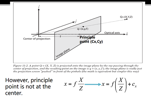
- Pinhole camera
- Because the point is not exactly at the center, we should add shift parameters and . So that .
- Why the aperture(孔径,光圈) cannot be too small?
- Less light passes through
- Diffraction effect
- Because the point is not exactly at the center, we should add shift parameters and . So that .
- Lenses
- For thin lense:
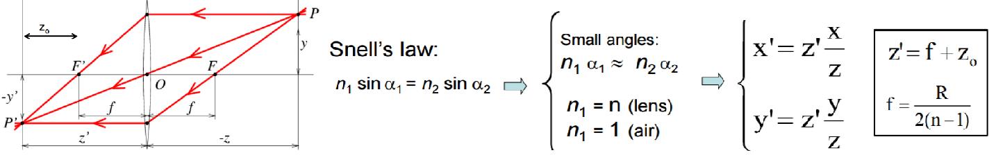
- For thin lense:
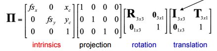
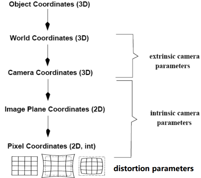
- intrinsic parameters
- From Pinhole Camera Model, totally parameters. Use the trick of Homogeneous Coordinates, finally:
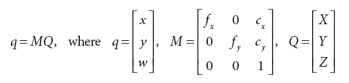
- From Pinhole Camera Model, totally parameters. Use the trick of Homogeneous Coordinates, finally:
- extrinsic parameters
- rotation and translation
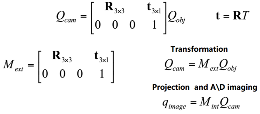
- parameters:
- rotation and translation
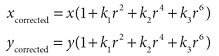
- distortion parameters
- Radial distortion
- caused by the geometry of the lens and aperture position.
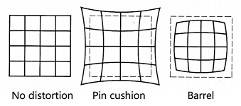
- caused by the geometry of the lens and aperture position.
- Tangential distortion
- caused by the decentering of the optical component (assembly process)
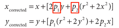
- parameters:
- caused by the decentering of the optical component (assembly process)
- Radial distortion
- Total Transformation
- Without distortion, the transform matrices are as follows:
- Steps
- Without distortion, the transform matrices are as follows:
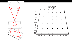
- Camera Calibration
- Compute relation between pixels and rays in space.
- Self-Calibration
- Do not use any calibration object. Moving camera in static scene.
- Very flexible, but not reliable
- 3D reference object-based Calibration
- Can be done very efficiently, but expensive calibration apparatus and elaborate setup required.
- Calibration by Homography
- Pros:
- Consider flexibility, robustness, and low cost.
- Only require the camera to observe a planar pattern shown at a few (minimum 2) different orientations.
- More flexible and robust than traditional techniques.
- 步骤:
- Calibration object: we know positions of corners of grid with respect to a coordinate system.
- Find the corners from images.
- Construct the equations.
- Solve the equations to get the camera parameters.
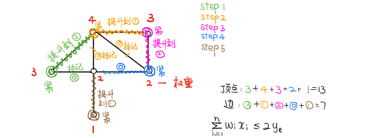
- 注意事项:
- 这个系统里有 个参数,但是二维图像变换的齐次坐标的自由度只有 。即若只有一组照片,取再多的点都不能求出所有参数。
- 假设取了 组图像,每组图像 个点,共获得了 个约束。
- 总参数是 ,则
- Pros:
Stereo Vision 立体视觉
- Triangulation
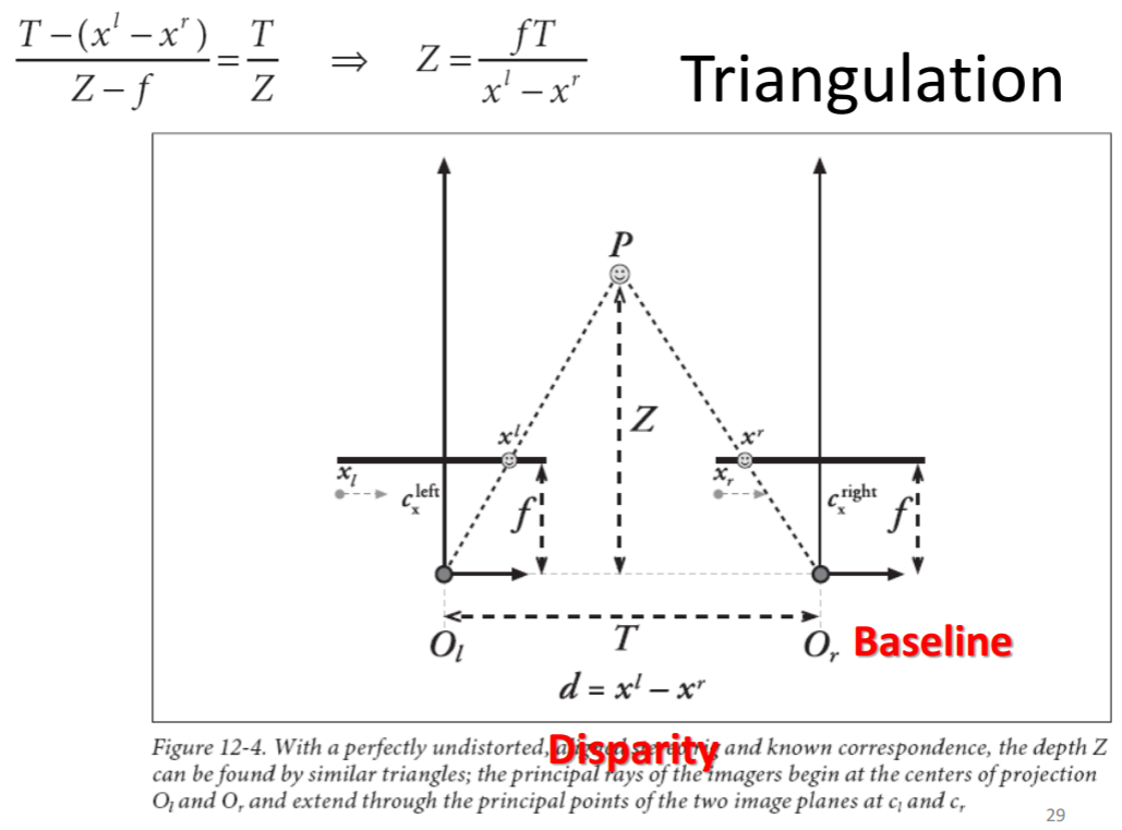
- 四个基本步骤
- Undistortion: remove distortions -> undistorted images.
- Rectification: adjust cameras -> the two images row-aligned
- Correspondence: find the same features in the two images -> disparity – Reprojection
- triangulation -> a depth map
图像分割
- Clustering: group together similar points and represent them with a single token
- Summarizing data
- Look at large amounts of data
- Patch-based compression or denoising
- Represent a large continuous vector with the cluster number
- Counting
- Histograms of texture, color, SIFT vectors
- Segmentation
- Separate the image into different regions
- Prediction
- Images in the same cluster may have the same labels.
- Summarizing data
- K-means algorithm
- Steps
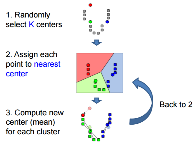
- Pros: Simple and fast; Easy to implement
- Cons: Need to choose K; Sensitive to outliers
- Steps
- Mean Shift
- The mean shift algorithm seeks modes of the given set of points.
- Steps:
- Choose kernel and bandwidth
- For each point: a) Center a window on that point b) Compute the mean of the data in the search window c) Center the search window at the new mean location d) Repeat (b,c) until convergence
- Assign points that lead to nearby modes to the same cluster
- Pros
- Good general-purpose segmentation
- Flexible in number and shape of regions
- Robust to outliers
- Cons
- Have to choose kernel size in advance
- Not suitable for high-dimensional features
All articles on this blog are licensed under CC BY-NC-SA 4.0 unless otherwise stated.
 wechat
 alipay
Related Articles
2023-07-27
算法的设计和分析
记录了我 2020.4-2020.6 在浙江大学上的《算法设计与分析》这门课的知识点。我会挑一些新奇有趣的、以前没见过的主题进行分享,可以把这篇文章和趣题摘记系列结合起来看。
2023-07-27
应用运筹学-线性规划应用
我在大三春夏学期上了张国川老师的《应用运筹学基础》这门课。张国川老师坚持板书讲解,课上干货满满,这篇文章是三分之一的课程笔记。
2023-07-27
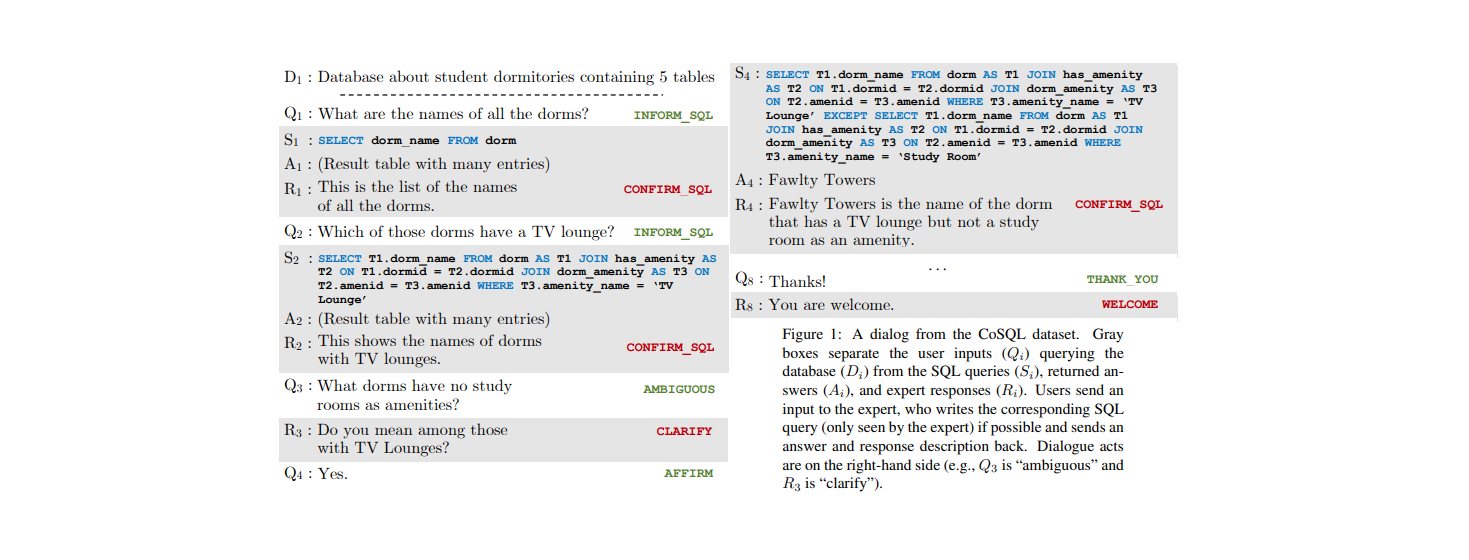
CoSQL 数据集
记录了我 2020.3-2020.6 在浙江大学上的《机器学习》这门课的知识点。
2021-09-05
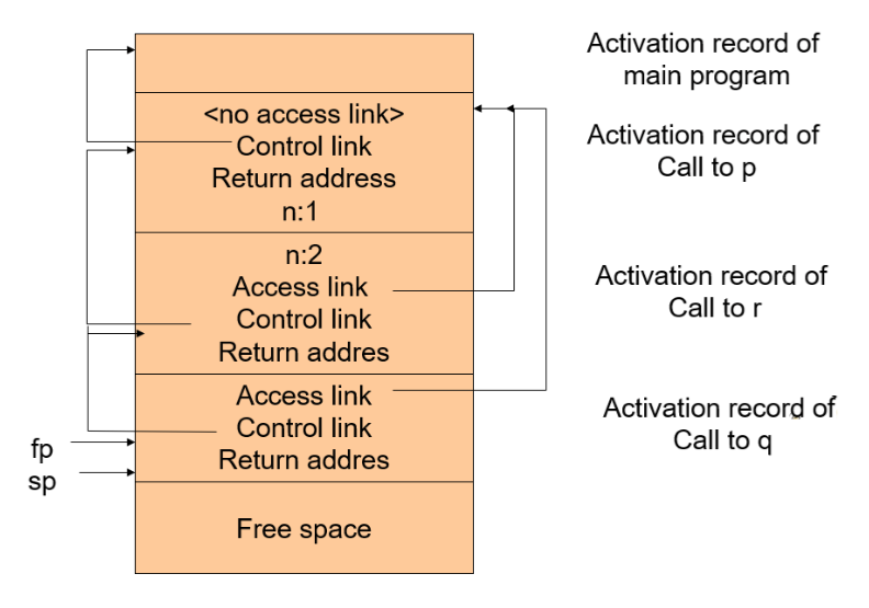
《编译原理》知识整理
记录了我 2020.3-2020.6 在浙江大学上的《编译原理》这门课的知识点。
2021-09-05
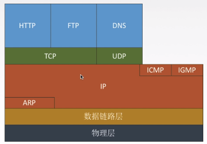
《计算机网络》知识整理
记录了我 2020.3-2020.6 在浙江大学上的《计算机网络》这门课的知识点。

2020-06-30
《计算机组成》知识整理
记录了我 2019.3-2019.6 在浙江大学上的《计算机组成》这门课的知识点。